基本搜索算法学习3
搜索算法
一个工作园区内存在多个仓库,不同的仓库内存放着不同的物品。现在从仓库中取出物体"A",但因为管理系统临时损坏,只能在园区不同仓库内查找.
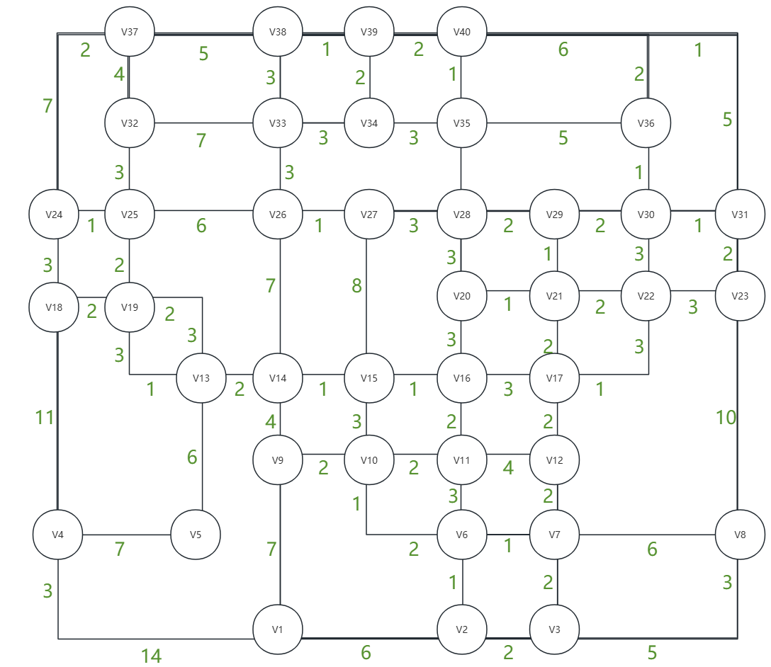
园区的仓库这样分布,其中v n 是 id 为 n-1 的仓库(例如:v1是id为0的仓库),边(edge)上数字是仓库之间联通的道路长度。

工人现在决定每到一个仓库就对仓库内所有点物品进行排查。如果安排排查的工人只有一人,该以怎样的顺序搜索才能最快找到A呢?
(⊙﹏⊙)我们将实际的邻接矩阵构建出来(M代表不邻接)。

假设A实际在仓库v37(id = 36),我们将点使用代码构建出来
originGraph ,optimizedGraph = graph_process.read_graph('original_graph.xlsx')
class Node:
    def __init__(self, id, position):
        self.id = id
        self.name = f"v{id+1}"
        self.position = None
        self.neighbor = []
        self.inhabitant = []
        if id == 36:
            self.inhabitant.append("A")
        self.f = 0
    def search(self,name):
        if name in self.inhabitant:
            return True
        else:
            return False

Nodes = {}
for i in range(len(originGraph)):
    node = Node(i, (0, 0))
    for j in range(len(originGraph)):
        if originGraph[i][j] != float('inf'):
            node.neighbor.append(j)
    Nodes[i] = node
start_node = 0
BFS
我们使用BFS搜索顺序进行搜查:
# we can use BFS to find the A
def BFS(start, target):
    # create a queue
    queue = []
    # create a list to store the visited nodes and the node which is planned to visit
    visited = [start]
    # create a list to store the path
    path = []
    # add the start node to the queue
    queue.append(start)
    # while the queue is not empty
    while queue:
        # get the first element in the queue
        node = queue.pop(0)
        # add the node to the path
        path.append(node)
        # if the node is the end node
        # search current node
        if Nodes[node].search(target):
            return path
        # get the neighbors of the node
        for neighbor_node in Nodes[node].neighbor:
            # if the node is not visited and the distance between the node and the neighbor is not infinite
            if neighbor_node not in visited:
                # add the neighbor to the queue
                queue.append(neighbor_node)
                visited.append(neighbor_node)
    return path # 得出搜索路径
path = BFS(start_node, "A")
print(f"BFS search_path:{path} \nlen:{len(path)}")
可以得到结果:
BFS search_path:[0, 1, 3, 8, 2, 5, 4, 17, 9, 13, 6, 7, 10, 12, 18, 23, 14, 25, 11, 22, 15, 24, 36]
len:23
工人使用BFS算法排查到第23个仓库才找到了A
DFS
现在我们使用DFS算法尝试寻找A
def DFS_recur(start, target, visited = [], path = []):
    visited.append(start)
    path.append(start)
    if Nodes[start].search(target):
        return path
    for neighbor_node in Nodes[start].neighbor:
        if neighbor_node not in visited:
            result = DFS_recur(neighbor_node, target, visited, path)
            if result:
                return result
    return None


def DFS_recur_post_order(start, target, visited = [], path = []):
    visited.append(start)
    for neighbor_node in Nodes[start].neighbor:
        if neighbor_node not in visited:
            result = DFS_recur_post_order(neighbor_node, target, visited, path)
            if result:
                return result
    path.append(start)
    if Nodes[start].search(target):
        return path
    return None
运行
path = DFS_recur(start_node, "A")
print(f"DFS_recur_preorder search_path:{path} \nlen:{len(path)}")

path = DFS_recur_post_order(start_node, "A")
print(f"DFS_recur_post_order search_path:{path} \nlen:{len(path)}")
得到结果
DFS_recur_preorder search_path:[0, 1, 2, 6, 5, 9, 8, 13, 12, 4, 3, 17, 18, 24, 23, 36]
len:16
DFS_recur_post_order search_path:[7, 37, 39, 38, 33, 34, 35, 40, 30, 22, 21, 29, 28, 27, 19, 20, 16, 11, 10, 15, 14, 26, 25, 32, 31, 36]
len:26
也就是说工人以先序深度优先搜索的顺序排查,可以在排查15个仓库后找到A。后序深度优先则更慢。
此时,运输设备停在出发点v1(id=0)等待工人找到A的位置后去将其运出。
假设工人并不熟悉园区的环境,即使找到了A货物所在的地点,也只能按照一路找来的仓库原路返回,再从出发点按照探索节点的顺序一路走到货物A所在节点。为了提高效率找到不绕圈的路径,工人使用了一致代价搜索。
# we can use Dijkstra to find the path
def UniformCostSearch(ori_graph, start, target):
    dist={} # record the distance from start to the node
    # record the previous node
    pred={}
    search_path = [start] # search_path use to record the order which the node is real visited
    if Nodes[start].search(target):
        path = [start]
        return search_path , path
    dist[start]=0
    while True:
        min = np.inf
        min_index = -1
        for visited_node in search_path:
            for neighbor_node in Nodes[visited_node].neighbor:
                if neighbor_node not in search_path and dist[visited_node] + ori_graph[visited_node][neighbor_node] < dist.get(neighbor_node, np.inf):
                    dist[neighbor_node] = dist[visited_node] + ori_graph[visited_node][neighbor_node]
                    pred[neighbor_node] = visited_node
                if neighbor_node not in search_path and dist[neighbor_node] <= min:
                    min = dist[neighbor_node]
                    min_index = neighbor_node
        search_path.append(min_index)
        if Nodes[min_index].search(target):
            print('find the end node')
            break
        if len(search_path) == len(Nodes):
            print('can not find the A')
            return search_path, []

    current = search_path[-1]
    path =[current] # real path form start to end
    while(current!=start):
        current = pred[current]
        path.insert(0,current)
    return path ,search_path
# run code
path ,search_path = UniformCostSearch(originGraph, 0, 'A')
print(f'Dijkstra_Path:{path}\nuniform cost search_path:{search_path}\nlen:{len(search_path)}')
得到结果
Dijkstra_Path:[0, 8, 13, 12, 18, 24, 31, 36]
uniform cost search_path:[0, 1, 5, 8, 6, 2, 9, 10, 11, 13, 14, 15, 16, 12, 20, 7, 28, 19, 21, 29, 27, 18, 3, 35, 30, 25, 26, 24, 22, 17, 4, 23, 40, 32, 34, 39, 31, 38, 37, 33, 36]
len:41 因此,一致代价搜索找到了从出发点到目标点的最短路径。
但是,使用UniformCost Search排查的顺序是按照距离出发点的顺序来的,正巧A所在的仓库v37是离仓库v1最远的点,因此是排查耗时最久,直至排查到最后一个仓库才找到了货物。也就是舍弃了排查成本而注重运输成本。
无信息搜索算法 结论
上述几个算法中,BFS和后序DFS搜索效果都不是特别好,先序DFS搜索可以节约排查成本,最快速的找到货物A所在地,但是没办法同时找出起点到目标所在点的合理路径。我们又通过一致代价搜索(DIJKSTRA)算法,找到目标点同时得出起点到目标点的最短路径,但这种算法寻找离起点远的对象时,排查效率极低。在规模更大的地图上,甚至难以找出结果。
有信息搜索算法
现实世界中,我们很少遇到没有信息盲目排查的情况,同时也难以接受找不到合理路径的结果。假如我们可以得到有关结果的信息,我们可以利用这个信息为启发,有方向的寻找。既要减少排查的成本,也要同时找到合理的路径减少运输的成本。
例如,现在我知道园区内仓库的分布有一定的规律,与目标货物A位置越接近的仓库,存放的货物与A就有越多的相似特征。
A*算法
使用A*算法:我们使用detect函数和heuristic启发函数模拟计算某个仓库货物与A货物的特征差异,距离A越远的仓库,返回的差异数值越大。工人每次从周围连接的几个仓库中选择差异数值最小的排查。
def detect(target):
    return 36

def heuristic(node, target):
    # 使用欧几里得距离作为启发式函数
    return np.linalg.norm(np.array(Nodes[node].position) - np.array(Nodes[target].position))

def trynext(graph, current_node, try_node, target_node):
    g_score = graph[current_node][try_node]
    h_score = heuristic(try_node, target_node)
    f_score = g_score + h_score
    return f_score

def A_star_search(graph, start, target):
    current_node = start
    path = [current_node]
    search_path = [current_node]
    while not Nodes[current_node].search(target):
        f_score = np.inf
        next_node = None
        for neighbor_node in Nodes[current_node].neighbor:
            if neighbor_node not in search_path:
                search_path.append(neighbor_node)
                f = trynext(graph, current_node, neighbor_node, detect(target))
                if f < f_score:
                    f_score = f
                    next_node = neighbor_node
        if next_node is None:
            print('can not find the A')
            break
        path.append(next_node)
        current_node = next_node
    return path,search_path

path  = A_star_search(originGraph, start_node, 'A')
print(f'path:{path}\nlen:{len(path)}\nsearchpath{search_path}\nlen:{len(search_path)}')
得到结果:
path:[0, 1, 5, 6, 11, 16, 20, 28, 27, 26, 25, 32, 33, 38, 37, 36]
len:16
这里的探索的节点十六个,但是探索的路径是一条实际可行的路径
对比Dijkstra算法和A*算法:
Dijkstra_Path:[0, 8, 13, 12, 18, 24, 31, 36]
uniform cost search_path:[0, 1, 5, 8, 6, 2, 9, 10, 11, 13, 14, 15, 16, 12, 20, 7, 28, 19, 21, 29, 27, 18, 3, 35, 30, 25, 26, 24, 22, 17, 4, 23, 40, 32, 34, 39, 31, 38, 37, 33, 36]
len:41
real path length:26.0
path:[0, 1, 5, 6, 11, 16, 20, 28, 27, 26, 25, 32, 33, 38, 37, 36]
len:16
real path length:35.0
可见A*虽然路径不是最优,但是他只探索了16个节点就找到了目标节点,排查成本上相较于代价一致算法要低上一倍不止,但是路径成本只差了不到1/3.
优化算法
管理系统修好后,有了全图视野
弗洛伊德算法
工人得到了全图视野后,也得到了邻接矩阵,但是现在工人师傅接到了新的任务:计算任意两仓库之间移动的最短路径长度。
def floydWarshall(graph):
    # 获取顶点的数量
    n = len(graph)
    # 初始化距离矩阵和路径矩阵
    dist = [row[:] for row in graph]
    # 执行Floyd-Warshall算法
    for k in range(n):  # 对于每一个顶点作为中间顶点
        for i in range(n):  # 遍历每一个起始顶点
            for j in range(n):  # 遍历每一个终点
                if dist[i][j] > dist[i][k] + dist[k][j]:
                    dist[i][j] = (int)(dist[i][k] + dist[k][j])
    return dist
读取邻接矩阵并根据弗洛伊德算法计算最短路长度,将其变为全连通矩阵:
df = pd.read_excel('data.xlsx', sheet_name=0,header=None)
# 将DataFrame中的所有'M'替换为numpy.inf
df.replace('M', M, inplace=True)
# 如果需要将数据转换为二维数组(numpy数组)
graph = np.copy(df.values)
# print(df)
dist= floydWarshall(df.values)
于是,工人解决了问题。
TSP模型结合贪婪算法
假设V5其实是整个园区的货物入口,现在新进一批货物在V5暂留,这批货物应该被分别运往不同仓库如下:
| 目标仓库(v) | 1 | 3 | 13 | 15 | 21 | 28 | 33 | 37 |
|---|---|---|---|---|---|---|---|---|
| 物资量(单位/t) | 4 | 5 | 8 | 3 | 2 | 6 | 7 | 2 |
每次从配送点v5出发,且配送员每次最多可以配送的物资量为4t。当配送员剩余可配送量为零时,认为配送员完成单次派送,返回配送点进行下一次配送,直至所有的物资都被送到指定仓库。求这一过程中总配送路程的最小值以及配送路径。
思路
已知配送员的配送起点、起点的单次最大物资量、需求点及需求点的需求量。出发点和终点都相同,且要使运输总路程最短,我们认为这是一个变形的TSP问题(也可以是VRP问题)。经过推理可以得出,若直接考虑离出发点最近的派送点,可能产生由于最远点需求较大不得不多次派送从而使总路径增大的问题。因此,通过以下步骤,可以合理规划配送路径并最小化总路径长度,同时确保各需求点的需求得到满足。
①初始化:
定义初始变量:设配送员的起点为物资点(C),每次配送的最大载重量为cap= 4t。获取所有需求点及其对应的需求量。初始化记录剩余需求量和路径总长度的变量。将所需要配送的点分为已选择点集和未选择点集,已选择点集中最初仅有出发点。
②选择能够一次性满足的需求点:
在当前所有需求点中,判断是否有需求量小于或等于cap的点。如果存在这样的点,则从中选择能与已选点集中所有点构成的tsp回路最短的需求点进行配送。更新该需求点的需求量并增加路径总长度。
③更新状态:
如果配送员还有剩余载物量且仍有符合条件的需求点,重复步骤 2。如果当前没有能够一次性满足的需求点,转到步骤4。
④处理需求量较大的点:
如果存在需求量超过cap的需求点,仍优先选择能与已选点集中所有点构成tsp回路最短的点。对该需求点进行部分满足,并更新需求量和路径长度。
⑤返回仓库:
每次完成单次配送任务后,需要返回仓库,并更新总路径长度。从仓库出发,重新开始下一次配送。
⑥终止条件:
当所有需求点的需求量均为零时,停止计算,并输出总路径长度。
代码实现
调用gurobi进行TSP建模求解
import gurobipy as gp
from gurobipy import GRB
import numpy as np
# tsp模型
def tsp(graph):
    model = gp.Model("tsp")
    model.setParam(GRB.Param.OutputFlag, 0)
    n = len(graph[0])
    # 定义决策变量
    x = model.addVars(n, n, vtype=GRB.BINARY, name="x")
    # 目标函数:最小化总距离
    z = gp.quicksum(x[i, j] * graph[i][j] for i in range(n) for j in range(n) if i != j)
    model.setObjective(z, GRB.MINIMIZE)
    # 约束条件
    # 每个节点只能离开一次
    for i in range(n):
        model.addConstr(gp.quicksum(x[i, j] for j in range(n) if i != j) == 1, name="out_{}".format(i))
    # 每个节点只能进入一次
    for j in range(n):
        model.addConstr(gp.quicksum(x[i, j] for i in range(n) if i != j) == 1, name="in_{}".format(j))
    for k in range(n):
        model.addConstr(gp.quicksum(x[i, k] for i in range(n) if i == k) == 0, name="fuck_{}".format(k))
    # 子回路约束
    u = model.addVars(n, lb=-GRB.INFINITY, ub=GRB.INFINITY, name="u")
    for i in range(n):
        for j in range(n):
            if i != j and i > 0 and j > 0:
                # 将辅助变量u与决策变量x连接起来
                model.addConstr(u[i] - u[j] + n * x[i, j] <= n - 1, "break_{}_{}".format(i, j))
    # 配置求解器并求解
    model.optimize()
    # 输出结果
    x_list=[]
    if model.status == GRB.OPTIMAL:
        # print(f"The optimal objective is {model.objVal}")
        for v in model.getVars():
            if v.X >= 0.5 and v.varName.startswith('x'):
                # print(f"{v.varName} : {v.X}")
                x_list.append(f"{v.varName}")
    else:
        print("No optimal solution found.")
        return None
    return model.objVal ,x_list
贪婪算法
G = np.loadtxt("opt_graph.txt") #使用弗洛伊德算法优化的全连通矩阵
OG = np.loadtxt("ori_graph.txt") # 原邻接矩阵

#配送中心为 v5
start = 4
capacity = 4
all_lenth=0
all_path = []
count=0
#需求节点为 v3 v5 v9 v12  [index, need]
need = [
    [0,4],
    [2,5],
    [12,8],
    [14,3],
    [20,2],
    [27,6],
    [32,7],
    [36,2]
]
while(need):
    overplus = capacity
    tspnow = [start]
    x_tsp = []
    ####断点检查
    print(f"*************从起点出发****************\n当前需求need([需求点,需求量]):\n{need}")
    flag = True
    while(overplus>0):
        max1 = [0, -1]  # [长度, need_index]
        max2 = [0, -1]
        min1 = [M, -1]
        min2 = [M, -1]
        for i in range(len(need)):
            if overplus >= need[i][1]:
                tsptry = tspnow.copy()
                tsptry.append(need[i][0])
                temp_g = [[0 for _ in range(len(tsptry))] for _ in range(len(tsptry))]
                for k in range(len(tsptry)):
                    for j in range(len(tsptry)):
                        temp_g[k][j] = G[tsptry[k]][tsptry[j]]
                pathlen, meiyy = optalg.tsp(temp_g)
                if max1[0] < pathlen:
                    max1[0] = pathlen
                    max1[1] = i
                if min1[0] > pathlen:
                    min1[0] = pathlen
                    min1[1] = i
            else:
                tsptry = tspnow.copy()
                tsptry.append(need[i][0])
                temp_g = [[0 for _ in range(len(tsptry))] for _ in range(len(tsptry))]
                for k in range(len(tsptry)):
                    for j in range(len(tsptry)):
                        temp_g[k][j] = G[tsptry[k]][tsptry[j]]
                pathlen, meiyy = optalg.tsp(temp_g)
                if max2[0] < pathlen:
                    max2[0] = pathlen
                    max2[1] = i
                if min2[0] > pathlen:
                    min2[0] = pathlen
                    min2[1] = i
        print(f"##overplus = {overplus},tspnow = {tspnow},need={need}")
        if min1[1] > -1:
            tspnow.append(need[min1[1]][0])
            overplus -= need[min1[1]][1]
            need.pop(min1[1])
            pass
        elif min2[1] > -1:
            # print(f"max2={max2[1]}")
            tspnow.append(need[min2[1]][0])
            need[min2[1]][1] -= overplus
            overplus = 0
            pass
        else:
            break
        print(f"##overplus = {overplus},tspnow = {tspnow},x_tsp = {x_tsp},need={need}")
    print(f"overplus = {overplus},tspnow = {tspnow},x_tsp = {x_tsp},need={need}")
    ##得到第一个tsp圈
    temp_g = [[0 for _ in range(len(tspnow))] for _ in range(len(tspnow))]
    for k in range(len(tspnow)):
        for j in range(len(tspnow)):
            temp_g[k][j] = G[tspnow[k]][tspnow[j]]
    length_temp,x_temp = optalg.tsp(temp_g)
    # print(f"x-temp={x_temp}")
    for i in x_temp:
        var_name, indices = i.split('[')
        indices = indices[:-1]  # 去掉最后一个']'字符
        x_tsp.append(tspnow[(int)(indices.split(',')[0])]) # 分割索引为列表
    x_tsp.append(start)
    full_path=[]
    for i in range(len(x_tsp)-1):
        full_path.extend(optalg.dijk(OG,x_tsp[i],x_tsp[i+1]))
    full_path.append(x_tsp[-1])
    all_lenth+=length_temp
    all_path.append(x_tsp)
    print(f"路长{length_temp},路径{x_tsp}\nfullpath:{full_path}")
    count+=1

print("**************************")
print(f"总长{all_lenth},圈数:{count},{all_path}")
结果均为节点的索引,故v1对应0,类推
| 圈数 | 路长 | 路径 |
|---|---|---|
| 1 | 18 | [4, 12, 13, 14, 13, 12, 4] |
| 2 | 49 | [4, 12, 13, 14, 15, 19, 20, 28, 27, 34, 39, 38, 37, 36, 31, 24, 18, 12, 4] |
| 3 | 38 | [4, 12, 13, 8, 0, 8, 13, 12, 4] |
| 4 | 12 | [4, 12, 4] |
| 5 | 32 | [4, 12, 13, 14, 15, 19, 27, 19, 15, 14, 13, 12, 4] |
| 6 | 32 | [4, 12, 13, 14, 15, 19, 27, 19, 15, 14, 13, 12, 4] |
| 7 | 41 | [4, 12, 13, 14, 15, 19, 27, 26, 25, 32, 25, 13, 12, 4] |
| 8 | 36 | [4, 12, 13, 25, 32, 25, 13, 12, 4] |
| 9 | 36 | [4, 12, 13, 14, 15, 10, 5, 6, 2, 6, 5, 9, 14, 13, 12, 4] |
| 10 | 36 | [4, 12, 13, 14, 15, 10, 5, 6, 2, 6, 5, 9, 14, 13, 12, 4] |
| 总和 | 330 | [ [4, 14, 12, 4], [4, 20, 36, 4], [4, 0, 4], [4, 12, 4], [4, 12, 27, 4], [4, 27, 4], [4, 27, 32, 4], [4, 32, 4], [4, 2, 4], [4, 2, 4] ] |
货物错位归仓问题
仓库管理人员在维护仓库时发现了部分货物错误入库,现在需要把错误入库的货物送回正确的仓库。错误入库的货物信息如下:
| 货物编号 | 所在仓库 | 正确仓库 |
|---|---|---|
| 0 | 4 | 0 |
| 1 | 5 | 14 |
| 2 | 18 | 32 |
| 3 | 25 | 36 |
| 4 | 40 | 27 |
| 5 | 11 | 14 |
| 6 | 6 | 8 |
| 7 | 6 | 8 |
| 8 | 7 | 8 |
| 9 | 8 | 40 |
| 10 | 9 | 8 |
| 11 | 10 | 22 |
| 12 | 11 | 22 |
| 13 | 29 | 36 |
| 14 | 35 | 36 |
现在工人师傅从V5出发,要将错误入库的货物送回正确的仓库,如何安排取货和送货的顺序高效完成任务呢?
条件假设
- 配送员在路上行驶的平均速度是40km/h;
- 配送过程不存在道路拥堵的状况;
- 配送过程的取货用时和货物归仓用时是随机的。这里我们假设都满足正态分布且取正值,其中,顾客响应时间满足标准差为0.5,均值为3的正态分布;物资取用时间是标准差0.5,均值为1的正态分布;
动态规划
因为动态规划会遇上指数爆炸的问题,因此我们假设配送师傅工作时间只有一个小时,也就是将送货时长超过60分钟的情况剪枝,并且每五秒钟输出一次当前最优解。
思路:
使用动态规划配合分支定界的剪枝算法来求解:以接单量n为阶段标志,接单的组合为状态标志。
1)初始化:
没有接单,阶段n=0,只有一种状态:接单组合为空。这个状态下,配送时长为0,小于截至时间,故可以通过这个状态发展下一个阶段的状态。
2)逐步增加订单:
n=1阶段下所有状态都由前一阶段的状态发展而来,再对这个阶段所有状态判断能否发展下一阶段的状态,进而发展下一阶段的各个状态。由此类推。
3)退出条件:
当发展至某一阶段所有的状态都不符合发展下一阶段状态的条件时,停止发展。
4)得到最优解:
从已发展的阶段中寻找阶段最大且符合条件的状态后,进而筛选耗时最短的状态作为最优解。
第三问则在第二问的基础上增加每个状态的效益的计算。下一个状态是否可以发展的条件则是在满足时间约束同时满足效益得到优化这一约束。
代码实现如下:
import math
import numpy as np
import optalg
import time
M = math.inf
start_time = time.time()
optresult=[] # {itercount:opt_status}
G = np.loadtxt("opt_graph.txt")
OG = np.loadtxt("ori_graph.txt")
# 等待错误货物取出的时间 min
def throw_wait(x=1):
    # 定义正态分布的参数:均值(mean),标准差(stddev)
    mean = 3  # 均值
    stddev = 0.6  # 标准差
    if x==0:
        return mean
    else:
        return max(0.1 ,np.random.normal(mean, stddev))
# 货物入库时间
waittime2 = 1
def pick_wait(x=1):
    # 定义正态分布的参数:均值(mean),标准差(stddev)
    mean = 1  # 均值
    stddev = 0.2  # 标准差
    if x==0:
        return mean
    else:
        return max(0.1 ,np.random.normal(mean, stddev))
#平均每分钟移动的距离 60km/h = 1km/min  40km/h = 0.667km/h
averspeed = 0.667
# 最后一单送达时间限制
limit_time = 60
def printresult(stage,opt_status,OG):
    for n,stagelist in stage.items():
        print(f"**************第{n}阶段:***************")
        count=1
        for status0 in stagelist:
            print(f"*****第{n}阶段状态{count}:")
            count+=1
            time0=status0.get("time")
            # list(status0.get("ReceviedOrder"))
            ifew = status0.get("active")
            bh = status0.get("ReceviedOrder")
            print(f"货物编号:{bh}\n完成订单最短耗时:{time0}\n能否额外接单{ifew}")
    print_opt(opt_status,OG)
def print_opt(opt_status,OG):
    print("***************opt*******************")
    print(opt_status)
    full_path=[]
    path0=[]
    path0.extend(opt_status.get("path"))
    for i in range(len(path0) - 1):
        full_path.extend(optalg.dijk(OG, path0[i], path0[i + 1]))
    full_path.append(path0[-1])
    print(f"fullpath:{full_path}")

def GetTime(start_time,opt_status,OG,itercount):
    T = time.time()
    if  T- start_time >= 5:
        if not hasattr(GetTime, 'last_run_time'):
            GetTime.last_run_time = T
            print("运行超过5s,输出当前最优结果:")
            print(f"当前迭代次数{itercount}")
            print_opt(opt_status,OG)
            print("程序继续运行,将会在最优解得到更新时输出")
        elif T - GetTime.last_run_time >= 5:
            print("当前最优结果:")
            print(f"当前迭代次数{itercount}")
            print_opt(opt_status, OG)
            print("程序继续运行...")
            GetTime.last_run_time = T
    return T


########################################Q1
# 出发位置为 v1 index=0
start = 4
# 可接订单列表[pick, throw]
# pick为取货点,throw为送货点
take_out = [
    [4,0],
    [5,14],
    [18,32],
    [25,36],
    [40,27],
    [11,14],
    [6,8], #0.06
    [6,8], # 1.4
    [7,8], # 10.777399063110352 seconds
    [8,40], #  13.456018447875977 seconds
    [9,8], # 15.147678852081299 seconds
    [10,22], # 16.096506595611572 seconds
    [11,22], # 29.35
    [12,36],
    [13,36],
    [14,36],
    [29,36],
    [35,36],
]
take_out_index = list(range(len(take_out)))
# opttakeout = []
# for i in take_out:
#     if not opttakeout:
#         for j in range(len(opttakeout)):
#             if opttakeout[j][0] == i[0] and opttakeout[j][1]==i[1]:
#                 opttakeout[2].append(j)
#             else:
#                 i.append([j])
#                 opttakeout.append(i)
#     else:
#         opttakeout.append([take_out[0],[0]])
# print(opttakeout)
##init
n=0
stage ={} # 放所有阶段 stage[0]就算n=0
allstatus =[] # 放本阶段包含的所有
opt_status={"time":0,"stage":0,"ReceviedOrder": set(),"active":True,"path":[]}
allstatus.append(opt_status)
stage[0] = allstatus
itercount = 0

##动态规划
while True:
    n+=1 #阶段数/单量
    if n>7:
        print("over6")
        break
    allstatus =[] #放本阶段包含的所有
    for prestage_statu in stage[n-1]:
        if not prestage_statu["active"]:
            continue
        # trystatus = prestage_statu
        canadd = list(set(take_out_index) - prestage_statu["ReceviedOrder"])
        for add_index in canadd:
            flag = False
            # new_get_index = prestage_statu.get("ReceviedOrder").copy().add(add_index)
            new_get_index = prestage_statu["ReceviedOrder"].copy()
            new_get_index.add(add_index)
            # print(new_get_index)
            for check in allstatus:
                if check.get("ReceviedOrder") == new_get_index:
                    flag = True
                    break
            if flag: #新的订单集合已经存在
                continue
            #新的订单集合不存在
            # print(new_get_index)
            dingdamn = [take_out[i] for i in new_get_index]
            newlenth,newpath = optalg.dpmin(G,start,dingdamn)
            newtime = (n-1)*throw_wait(0)+ newlenth/averspeed +n*pick_wait(0)
            estimatedtime = (n-1)*throw_wait()+ newlenth/averspeed +n*pick_wait()
            if newtime < limit_time:
                newstatus = {"time": newtime,"estimatedtime":estimatedtime, "stage": n, "ReceviedOrder": new_get_index, "active": True,"path":newpath}
            else:
                newstatus = {"time": newtime,"estimatedtime":estimatedtime,  "stage": n, "ReceviedOrder": new_get_index, "active": False,"path":newpath}
            # 找最优
            itercount+=1
            temptime = GetTime(start_time, opt_status, OG, itercount) - start_time
            if newstatus.get("time")<=limit_time and newstatus.get("stage")>=opt_status.get("stage"):
                # if newstatus.get("stage")>opt_status.get("stage"):
                opt_status = newstatus
                optresult.append(f"接单数{n},迭代次数{itercount},运行至此耗时{round(temptime,2)}s")
                # elif newstatus.get("time")<opt_status.get("time"):
                #     opt_status = newstatus
                    # optresult.append(f"接单数{n},迭代次数{itercount},运行至此耗时{round(temptime, 2)}s")
            allstatus.append(newstatus)
    # print(allstatus)
    if not allstatus:
        break
    stage[n]=allstatus
printresult(stage,opt_status,OG)
print(f"exc:{time.time()-start_time}")
for i in optresult:
    print(i)
于是得到结果
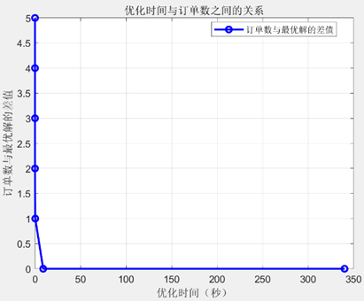
因为动态规划状态数增长太快,因此设置每五秒钟输出一次答案。以便观察优化结果:
运行超过5s,输出当前最优结果:
当前迭代次数1326
***************opt*******************
{'time': 54.97901049475262, 'estimatedtime': 53.528791967788415, 'stage': 4, 'ReceviedOrder': {10, 5, 6, 7}, 'active': True, 'path': [4, 11, 6, 6, 9, 8, 8, 8, 14]}
fullpath:[4, 12, 13, 14, 15, 16, 11, 6, 5, 9, 8, 9, 14]
程序继续运行,将会在最优解得到更新时输出
当前最优结果:
当前迭代次数1346
***************opt*******************
{'time': 54.97901049475262, 'estimatedtime': 53.528791967788415, 'stage': 4, 'ReceviedOrder': {10, 5, 6, 7}, 'active': True, 'path': [4, 11, 6, 6, 9, 8, 8, 8, 14]}
fullpath:[4, 12, 13, 14, 15, 16, 11, 6, 5, 9, 8, 9, 14]
程序继续运行...
当前最优结果:
当前迭代次数1363
***************opt*******************
{'time': 58.97901049475262, 'estimatedtime': 60.7242975447131, 'stage': 5, 'ReceviedOrder': {1, 5, 6, 7, 10}, 'active': True, 'path': [4, 11, 6, 6, 5, 9, 8, 8, 8, 14, 14]}
fullpath:[4, 12, 13, 14, 15, 16, 11, 6, 5, 9, 8, 9, 14]
程序继续运行...
......
运行结果
运行程序,可以得出接单数量与迭代次数,接单数量与运行用时之间的关系如下表所示:
| 接单数 | 迭代次数 | 运行至此耗时 |
|---|---|---|
| 1 | 1 | 0.0s |
| 2 | 19 | 0.0s |
| 3 | 180 | 0.01s |
| 4 | 820 | 0.3s |
| 5 | 1356 | 8.97s |
将已接单数目与运行时间和迭代次数之间的关系分别可视化,具体关系如下图所示 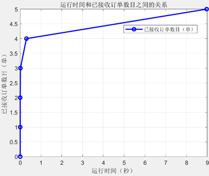
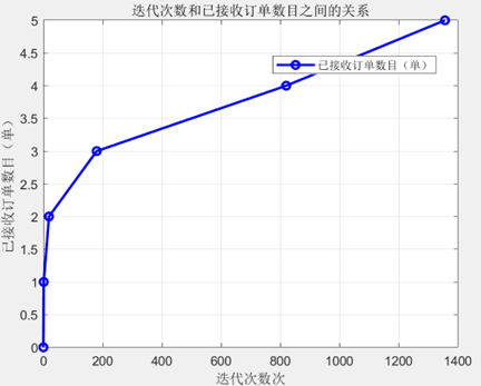
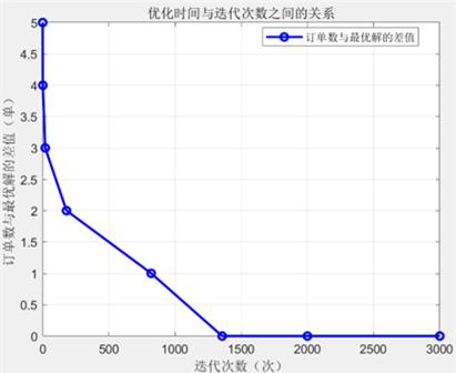
由运行结果可知在不超过截止时间的前提下,他最多一次性能接5单,接编号为1、5、6、7、10的订单,取餐送餐路线为:4, 12, 13, 14, 15, 16, 11, 6, 5, 9, 8, 9, 14,预计到达最后一个送货点所在地需要58.98分钟.
假如我要全部送完,那动态规划遭遇了指数爆炸,肯定没戏了,因此我们可以使用:
遗传算法
直接上代码:
import random
from copy import deepcopy
from collections import Counter

import numpy as np
from tqdm import tqdm

import graph_process

originGraph ,optimizedGraph = graph_process.read_graph('original_graph.xlsx')
start = 4
take_out = [
    [4,0],
    [5,14],
    [18,32],
    [25,36],
    [40,27],
    [11,14],
    [6,8],
    [6,8],
    [7,8],
    [8,40],
    [9,8],
    [10,22],
    [11,22],
    [12,36],
    [13,36],
    [14,36],
    [29,36],
    [35,36],
]
alldata = []
for i in take_out:
    alldata.append(i[0])
    alldata.append(i[1])
element_counts = Counter(alldata)
# Convert to dictionary
element_counts_dict = dict(element_counts)
print(element_counts_dict)

VARY = 0.05  # 变异几率
class Gene:
    def __init__(self, name='Gene', data=None):
        self.name = name
        self.length =2*len(take_out)
        if data is None:
            self.data = self._getGene()
        else:
            self.data = data
        self.giggity = None
        self.fit = self.getFit()
        self.chooseProb = 0  # 选择概率

    def _getGene(self):
        data = []
        for i in take_out:
            data.append(i[0])
            data.append(i[1])
        random.shuffle(data)
        return data

    # return fitness
    def getFit(self):
        fit = 0
        order_list = take_out.copy()
        get_order = []
        self.giggity = []
        for i in self.data:
            tempLog = []
            tempLog.append(["到达", i])
            poplist = []
            for j in range(len(order_list)):
                if i == order_list[j][0]:
                    poplist.append(j)
                    tempLog.append(["装货", order_list[j]])
            for j in range(len(poplist)):
                get_order.append(order_list.pop(poplist[j]-j))
            poplist.clear()
            for j in range(len(get_order)):
                if i == get_order[j][1]:
                    poplist.append(j)
                    tempLog.append(["卸货", get_order[j]])
            for j in range(len(poplist)):
                get_order.pop(poplist[j]-j)
            if len(tempLog) != 1:
                self.giggity.append(tempLog)


        if len(order_list) != 0:
            self.giggity = 'error'
        elif len(get_order) != 0:
            fit += np.inf
            self.giggity = 'error'

        dist = []  # from this to next
        # calculate distance
        i = 1
        while i < len(self.data):
            v1 = self.data[i - 1]
            v2 = self.data[i]
            dist.append(optimizedGraph[v1][v2])
            i += 1

        # distance cost
        distCost = sum(dist)+optimizedGraph[start][self.data[0]]

        fit += distCost
        return 1/fit

    def updateChooseProb(self, sumFit):
        self.chooseProb = self.fit / sumFit

    def moveRandSubPathLeft(self):
        path = random.randrange(len(self.data))  # choose a path index
        swapped_list = self.data[path:] + self.data[:path]
        self.data = swapped_list

# return a bunch of random genes
def getRandomGenes(size):
    genes = []
    for i in range(size):
        genes.append(Gene("Gene "+str(i)))
    return genes

def getSumFit(genes):
    sumFit = 0
    for gene in genes:
        sumFit += gene.fit
    return sumFit

def updateChooseProb(genes):
    sumFit = getSumFit(genes)
    for gene in genes:
        gene.updateChooseProb(sumFit)

# 计算累计概率
def getSumProb(genes):
    sum = 0
    for gene in genes:
        sum += gene.chooseProb
    return sum

# 选择复制,选择前 1/3
def choose(genes):
    num = int(geneNum/6) * 2    # 选择偶数个,方便下一步交叉
    # sort genes with respect to chooseProb
    key = lambda gene: gene.chooseProb
    genes.sort(reverse=True, key=key)
    # return shuffled top 1/3
    return genes[0:num]

# 交叉一对
def crossPair(gene1, gene2, crossedGenes):
    gene1.moveRandSubPathLeft()
    gene2.moveRandSubPathLeft()
    key = lambda gene: gene.fit

    possible = []
    for _ in range(10):
        newGene1 = []
        p1= random.randrange(len(gene1.data))
        p2 = 0
        tempdict = element_counts_dict.copy()
        while p2 != p1:
            ele = gene1.data[p2]
            newGene1.append(ele)
            tempdict[ele] -= 1
            p2 += 1
        # copy data not exits in father gene
        for pos in gene2.data:
            if tempdict[pos] > 0:
                tempdict[pos] -= 1
                newGene1.append(pos)
        possible.append(Gene(data=newGene1))
    possible.sort(reverse=True, key=key)
    crossedGenes.append(possible[0])
    possible = []
    for _ in range(10):
        newGene2 = []
        p1 = random.randrange(len(gene2.data))
        p2 = 0
        tempdict = element_counts_dict.copy()
        while p2 != p1:
            ele = gene1.data[p2]
            newGene2.append(ele)
            tempdict[ele] -= 1
            p2 += 1
        # copy data not exits in father gene
        for pos in gene1.data:
            if tempdict[pos] > 0:
                tempdict[pos] -= 1
                newGene2.append(pos)
        possible.append(Gene(data=newGene2))
    possible.sort(reverse=True, key=key)
    crossedGenes.append(possible[0])


# 交叉
def cross(genes):
    crossedGenes = []
    for i in range(0, len(genes), 2):
        crossPair(genes[i], genes[i+1], crossedGenes)
    return crossedGenes

# 合并
def mergeGenes(genes, crossedGenes):
    # sort genes with respect to chooseProb
    key = lambda gene: gene.chooseProb
    genes.sort(reverse=True, key=key)
    pos = geneNum - 1
    for gene in crossedGenes:
        genes[pos] = gene
        pos -= 1
    return  genes

# 变异一个
def varyOne(gene):
    varyNum = 10
    variedGenes = []
    for i in range(varyNum):
        p1, p2 = random.choices(list(range(1,len(gene.data)-2)), k=2)
        newGene = gene.data.copy()
        newGene[p1], newGene[p2] = newGene[p2], newGene[p1] # 交换
        variedGenes.append(Gene(data=newGene.copy()))
    key = lambda gene: gene.fit
    variedGenes.sort(reverse=True, key=key)
    return variedGenes[0]

# 变异
def vary(genes):
    for index, gene in enumerate(genes):
        # 精英主义,保留前三十
        if index < 30:
            continue
        if random.random() < VARY:
            genes[index] = varyOne(gene)
    return genes


if __name__ == "__main__" :

    geneNum = 100
    generationNum = 3000  # 迭代次数
    genes = getRandomGenes(geneNum) # 初始种群
    # 迭代
    for i in tqdm(range(generationNum)):
        updateChooseProb(genes)
        # sumProb = getSumProb(genes)
        chosenGenes = choose(deepcopy(genes))   # 选择
        crossedGenes = cross(chosenGenes)   # 交叉
        genes = mergeGenes(genes, crossedGenes) # 复制交叉至子代种群
        genes = vary(genes) # under construction
    # sort genes with respect to chooseProb
    key = lambda gene: gene.fit
    genes.sort(reverse=True, key=key)   # 以fit对种群排序
    print('\r\n')
    print('data:', genes[0].data)
    print('fit:', genes[0].fit)
    print(f'从{start}到出发')
    for i in genes[0].giggity:
        for j in i:
            if j[0] != '到达':
                index = take_out.index(j[1])
                print(f'{j[0]}:任务编号{index}')
            else:
                print(f'{j[0]}:{j[1]}')
结果
可以得到整个任务的最优解:
data: [4, 12, 35, 29, 11, 11, 6, 6, 7, 5, 10, 14, 9, 0, 8, 8, 8, 8, 8, 13, 14, 14, 22, 22, 40, 40, 27, 25, 18, 36, 36, 36, 36, 36, 36, 32]
fit: 0.008130081300813009
从4到出发
到达:4
装货:任务编号0
到达:12
装货:任务编号13
到达:35
装货:任务编号17
到达:29
装货:任务编号16
到达:11
装货:任务编号5
装货:任务编号12
到达:6
装货:任务编号6
装货:任务编号6
到达:7
装货:任务编号8
到达:5
装货:任务编号1
到达:10
装货:任务编号11
到达:14
装货:任务编号15
卸货:任务编号5
卸货:任务编号1
到达:9
装货:任务编号10
到达:0
卸货:任务编号0
到达:8
装货:任务编号9
卸货:任务编号6
卸货:任务编号6
卸货:任务编号8
卸货:任务编号10
到达:13
装货:任务编号14
到达:22
卸货:任务编号12
卸货:任务编号11
到达:40
装货:任务编号4
卸货:任务编号9
到达:27
卸货:任务编号4
到达:25
装货:任务编号3
到达:18
装货:任务编号2
到达:36
卸货:任务编号13
卸货:任务编号17
卸货:任务编号16
卸货:任务编号15
卸货:任务编号14
卸货:任务编号3
到达:32
卸货:任务编号2
最优性比较
为了比较遗传算法的优化性能,我们将任务列表删减为动态规划得出的最优解,比较两种算法的结果差异:
遗传算法
省略了出发站点4
data: [11, 6, 6, 5, 9, 8, 8, 8, 14, 14]
fit: 0.03571428571428571
从4到出发
到达:11
装货:任务编号1
到达:6
装货:任务编号2
装货:任务编号2
到达:5
装货:任务编号0
到达:9
装货:任务编号4
到达:8
卸货:任务编号2
卸货:任务编号2
卸货:任务编号4
到达:14
卸货:任务编号1
卸货:任务编号0
动态规划
看path
***************opt*******************
{'time': 58.97901049475262, 'estimatedtime': 60.7242975447131, 'stage': 5, 'ReceviedOrder': {1, 5, 6, 7, 10}, 'active': True, 'path': [4, 11, 6, 6, 5, 9, 8, 8, 8, 14, 14]}
fullpath:[4, 12, 13, 14, 15, 16, 11, 6, 5, 9, 8, 9, 14]
结论
显然两种算法小规模的解一致,但动态规划算法求解受到规模约束,而遗传算法不会。因此遗传算法更优越。
禁忌搜索
# Function: Tabu Search Demo
import random
import numpy as np
import graph_process
from tqdm import tqdm

# 输入条件
# input condition
start = 4
take_out = [
    [4,0],
    [5,14],
    [18,32],
    [25,36],
    [40,27],
    [11,14],
    [6,8],
    [6,8],
    [7,8],
    [8,40],
    [9,8],
    [10,22],
    [11,22],
    [12,36],
    [13,36],
    [14,36],
    [29,36],
    [35,36],
]


# setting parameters
length_tabulist = 40
candidate_number = 300
loop_times = 3000
tabu_list = []
solution_record = []
originGraph ,optimizedGraph = graph_process.read_graph('original_graph.xlsx')

class Solution:
    def __init__(self, data = None , action = None):
        if data is None:
            self.data = self._get_original_salution()
        else:
            self.data = data
        self.cost = self.get_cost()
        self.action = action
        self.giggity = [] #记录操作流程
    def get_cost(self):
        cost = 0
        order_list = take_out.copy()
        get_order = []
        self.giggity = []
        for i in self.data:
            tempLog = []
            tempLog.append(["到达", i])
            poplist = []
            for j in range(len(order_list)):
                if i == order_list[j][0]:
                    poplist.append(j)
                    tempLog.append(["装货", order_list[j]])
            for j in range(len(poplist)):
                get_order.append(order_list.pop(poplist[j]-j))
            poplist.clear()
            for j in range(len(get_order)):
                if i == get_order[j][1]:
                    poplist.append(j)
                    tempLog.append(["卸货", get_order[j]])
            for j in range(len(poplist)):
                get_order.pop(poplist[j]-j)
            if len(tempLog) != 1:
                self.giggity.append(tempLog)

        if len(order_list) != 0:
            self.giggity = 'error'
        elif len(get_order) != 0:
            cost += np.inf
            self.giggity = 'error'

        dist = []  # from this to next
        # calculate distance
        i = 1
        while i < len(self.data):
            v1 = self.data[i - 1]
            v2 = self.data[i]
            dist.append(optimizedGraph[v1][v2])
            i += 1

        # distance cost
        distCost = sum(dist)+optimizedGraph[start][self.data[0]]

        cost += distCost
        return cost

    def _get_original_salution(self):
        data = []
        for i in take_out:
            data.append(i[0])
            data.append(i[1])
        random.shuffle(data)
        return data


    def reverse(self, a, b):
        # 翻转索引a到b-1之间的城市
        self.data = self.data[:a] + self.data[a:b][::-1] + self.data[b:]
        return (0, a, b)
    def swap(self, a, b):
        # 交换两个城市的位置
        self.data[a], self.data[b] = self.data[b], self.data[a]
        return (1, a, b)
    def move(self, a, b):
        # 将城市a移动到城市b之后
        self.data.insert(b+1, self.data.pop(a))
        return (2, a, b)
    def get_neighborhood(self):
        # 随机选择两个城市
        a, b = random.sample(range(len(self.data)), 2)
        option = random.randint(0, 2)
        return (option, a, b)
    def generate_candidate(self , action):
        # 生成候选解
        option , a, b = action
        if option == 0:
            self.reverse(a, b)
        elif option == 1:
            self.swap(a, b)
        else:
            self.move(a, b)
        self.action = action
        self.cost = self.get_cost()


def optimize_solution(best_solution:Solution):
    global tabu_list ,solution_record
    current_solution = best_solution
    posible_solution = [current_solution]
    if len(tabu_list) > length_tabulist:
        for i in range(int(len(tabu_list)/5)):
            tabu_list.pop(i)
    for _ in range(candidate_number):
        new_solution = Solution(current_solution.data)
        neighbor = new_solution.get_neighborhood()
        if neighbor not in tabu_list:
            new_solution.generate_candidate(neighbor)
            if new_solution.cost < current_solution.cost:
                current_solution = new_solution
                posible_solution.append(current_solution)
            continue
    # choose the best solution form the posible_solution
    choose_solution = min(posible_solution, key=lambda x: x.cost)
    if choose_solution.action is not None:
        tabu_list.append(choose_solution.action)
        solution_record.append(choose_solution)
    else:
        print('No neighbor found')
    return choose_solution

if __name__ == "__main__" :
    best_solution =Solution()
    for i in tqdm(range(loop_times)):
        best_solution = optimize_solution(best_solution)
    print(best_solution.data)
    print(best_solution.cost)
    print(best_solution.giggity)
    for i in best_solution.giggity:
        for j in i:
            if j[0] != '到达':
                index = take_out.index(j[1])
                print(f'{j[0]}:任务编号{index}')
            else:
                print(f'{j[0]}:{j[1]}')
得到结果:
Tabu Search Progress: 100%|██████████| 30000/30000 [00:44<00:00, 679.04it/s]
Best Solution Data: [22, 25, 11, 36, 9, 12, 10, 8, 18, 8, 6, 11, 5, 35, 7, 13, 40, 36, 8, 14, 32, 4, 8, 36, 36, 27, 36, 14, 29, 22, 14, 40, 36, 0]
Best Solution Cost: 390.0
Operation Log:
Total Time Taken: 0:00:44.206928
可见优化后总路程为294
对比遗传算法,结果并不能更好,而且效率也不够高。
完整代码
BFS,DFS,A*,DIJKSTRA,UNICOST算法完整代码:
SearchMethod/SearchMethods_demo1.py at main · 57Darling02/SearchMethod (github.com)
TSP启发算法:
DeliveryKing/Q1.py at main · 57Darling02/DeliveryKing (github.com)
动态规划:
DeliveryKing/Q2.py at main · 57Darling02/DeliveryKing (github.com)
GA算法:
SearchMethod/GA_Demo2.py at main · 57Darling02/SearchMethod (github.com)
更多数据结构与算法:(多语言实现)